37. Samuelson Multiplier-Accelerator#
In addition to what’s in Anaconda, this lecture will need the following libraries:
!pip install quantecon
37.1. Overview#
This lecture creates non-stochastic and stochastic versions of Paul Samuelson’s celebrated multiplier accelerator model [Samuelson, 1939].
In doing so, we extend the example of the Solow model class in our second OOP lecture.
Our objectives are to
provide a more detailed example of OOP and classes
review a famous model
review linear difference equations, both deterministic and stochastic
Let’s start with some standard imports:
import matplotlib.pyplot as plt
import numpy as np
We’ll also use the following for various tasks described below:
from quantecon import LinearStateSpace
import cmath
import math
import sympy
from sympy import Symbol, init_printing
from cmath import sqrt
37.1.1. Samuelson’s model#
Samuelson used a second-order linear difference equation to represent a model of national output based on three components:
a national output identity asserting that national output or national income is the sum of consumption plus investment plus government purchases.
a Keynesian consumption function asserting that consumption at time \(t\) is equal to a constant times national output at time \(t-1\).
an investment accelerator asserting that investment at time \(t\) equals a constant called the accelerator coefficient times the difference in output between period \(t-1\) and \(t-2\).
Consumption plus investment plus government purchases constitute aggregate demand, which automatically calls forth an equal amount of aggregate supply.
(To read about linear difference equations see here or chapter IX of [Sargent, 1987].)
Samuelson used the model to analyze how particular values of the marginal propensity to consume and the accelerator coefficient might give rise to transient business cycles in national output.
Possible dynamic properties include
smooth convergence to a constant level of output
damped business cycles that eventually converge to a constant level of output
persistent business cycles that neither dampen nor explode
Later we present an extension that adds a random shock to the right side of the national income identity representing random fluctuations in aggregate demand.
This modification makes national output become governed by a second-order stochastic linear difference equation that, with appropriate parameter values, gives rise to recurrent irregular business cycles.
(To read about stochastic linear difference equations see chapter XI of [Sargent, 1987].)
37.2. Details#
Let’s assume that
\(\{G_t\}\) is a sequence of levels of government expenditures – we’ll start by setting \(G_t = G\) for all \(t\).
\(\{C_t\}\) is a sequence of levels of aggregate consumption expenditures, a key endogenous variable in the model.
\(\{I_t\}\) is a sequence of rates of investment, another key endogenous variable.
\(\{Y_t\}\) is a sequence of levels of national income, yet another endogenous variable.
\(\alpha\) is the marginal propensity to consume in the Keynesian consumption function \(C_t = \alpha Y_{t-1} + \gamma\).
\(\beta\) is the “accelerator coefficient” in the “investment accelerator” \(I_t = \beta (Y_{t-1} - Y_{t-2})\).
\(\{\epsilon_{t}\}\) is an IID sequence standard normal random variables.
\(\sigma \geq 0\) is a “volatility” parameter — setting \(\sigma = 0\) recovers the non-stochastic case that we’ll start with.
The model combines the consumption function
with the investment accelerator
and the national income identity
The parameter \(\alpha\) is peoples’ marginal propensity to consume out of income - equation (37.1) asserts that people consume a fraction of \(\alpha \in (0,1)\) of each additional dollar of income.
The parameter \(\beta > 0\) is the investment accelerator coefficient - equation (37.2) asserts that people invest in physical capital when income is increasing and disinvest when it is decreasing.
Equations (37.1), (37.2), and (37.3) imply the following second-order linear difference equation for national income:
or
where \(\rho_1 = (\alpha+\beta)\) and \(\rho_2 = -\beta\).
To complete the model, we require two initial conditions.
If the model is to generate time series for \(t=0, \ldots, T\), we require initial values
We’ll ordinarily set the parameters \((\alpha,\beta)\) so that starting from an arbitrary pair of initial conditions \((\bar Y_{-1}, \bar Y_{-2})\), national income \(Y_t\) converges to a constant value as \(t\) becomes large.
We are interested in studying
the transient fluctuations in \(Y_t\) as it converges to its steady state level
the rate at which it converges to a steady state level
The deterministic version of the model described so far — meaning that no random shocks hit aggregate demand — has only transient fluctuations.
We can convert the model to one that has persistent irregular fluctuations by adding a random shock to aggregate demand.
37.2.1. Stochastic version of the model#
We create a random or stochastic version of the model by adding a random process of shocks or disturbances \(\{\sigma \epsilon_t \}\) to the right side of equation (37.4), leading to the second-order scalar linear stochastic difference equation:
37.2.2. Mathematical analysis of the model#
To get started, let’s set \(G_t \equiv 0\), \(\sigma = 0\), and \(\gamma = 0\).
Then we can write equation (37.5) as
or
To discover the properties of the solution of (37.6), it is useful first to form the characteristic polynomial for (37.6):
where \(z\) is possibly a complex number.
We want to find the two zeros (a.k.a. roots) – namely \(\lambda_1, \lambda_2\) – of the characteristic polynomial.
These are two special values of \(z\), say \(z= \lambda_1\) and \(z= \lambda_2\), such that if we set \(z\) equal to one of these values in expression (37.7), the characteristic polynomial (37.7) equals zero:
Equation (37.8) is said to factor the characteristic polynomial.
When the roots are complex, they will occur as a complex conjugate pair.
When the roots are complex, it is convenient to represent them in the polar form
where \(r\) is the amplitude of the complex number and \(\omega\) is its angle or phase.
These can also be represented as
(To read about the polar form, see here)
Given initial conditions \(Y_{-1}, Y_{-2}\), we want to generate a solution of the difference equation (37.6).
It can be represented as
where \(c_1\) and \(c_2\) are constants that depend on the two initial conditions and on \(\rho_1, \rho_2\).
When the roots are complex, it is useful to pursue the following calculations.
Notice that
The only way that \(Y_t\) can be a real number for each \(t\) is if \(c_1 + c_2\) is a real number and \(c_1 - c_2\) is an imaginary number.
This happens only when \(c_1\) and \(c_2\) are complex conjugates, in which case they can be written in the polar forms
So we can write
where \(v\) and \(\theta\) are constants that must be chosen to satisfy initial conditions for \(Y_{-1}, Y_{-2}\).
This formula shows that when the roots are complex, \(Y_t\) displays oscillations with period \(\check p = \frac{2 \pi}{\omega}\) and damping factor \(r\).
We say that \(\check p\) is the period because in that amount of time the cosine wave \(\cos(\omega t + \theta)\) goes through exactly one complete cycles.
(Draw a cosine function to convince yourself of this please)
Remark: Following [Samuelson, 1939], we want to choose the parameters \(\alpha, \beta\) of the model so that the absolute values (of the possibly complex) roots \(\lambda_1, \lambda_2\) of the characteristic polynomial are both strictly less than one:
Remark: When both roots \(\lambda_1, \lambda_2\) of the characteristic polynomial have absolute values strictly less than one, the absolute value of the larger one governs the rate of convergence to the steady state of the non stochastic version of the model.
37.2.3. Things this lecture does#
We write a function to generate simulations of a \(\{Y_t\}\) sequence as a function of time.
The function requires that we put in initial conditions for \(Y_{-1}, Y_{-2}\).
The function checks that \(\alpha, \beta\) are set so that \(\lambda_1, \lambda_2\) are less than unity in absolute value (also called “modulus”).
The function also tells us whether the roots are complex, and, if they are complex, returns both their real and complex parts.
If the roots are both real, the function returns their values.
We use our function written to simulate paths that are stochastic (when \(\sigma >0\)).
We have written the function in a way that allows us to input \(\{G_t\}\) paths of a few simple forms, e.g.,
one time jumps in \(G\) at some time
a permanent jump in \(G\) that occurs at some time
We proceed to use the Samuelson multiplier-accelerator model as a laboratory to make a simple OOP example.
The “state” that determines next period’s \(Y_{t+1}\) is now not just the current value \(Y_t\) but also the once lagged value \(Y_{t-1}\).
This involves a little more bookkeeping than is required in the Solow model class definition.
We use the Samuelson multiplier-accelerator model as a vehicle for teaching how we can gradually add more features to the class.
We want to have a method in the class that automatically generates a simulation, either non-stochastic (\(\sigma=0\)) or stochastic (\(\sigma > 0\)).
We also show how to map the Samuelson model into a simple instance of the LinearStateSpace class described here.
We can use a LinearStateSpace instance to do various things that we did above with our homemade function and class.
Among other things, we show by example that the eigenvalues of the matrix \(A\) that we use to form the instance of the LinearStateSpace class for the Samuelson model equal the roots of the characteristic polynomial (37.7) for the Samuelson multiplier accelerator model.
Here is the formula for the matrix \(A\) in the linear state space system in the case that government expenditures are a constant \(G\):
37.3. Implementation#
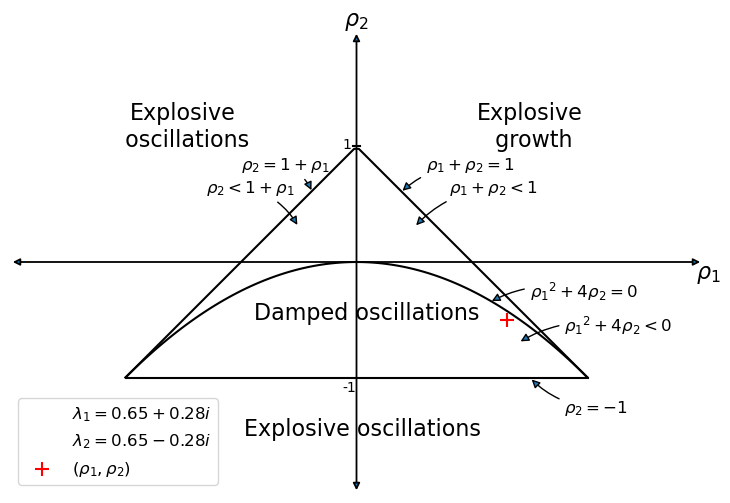
We’ll start by drawing an informative graph from page 189 of [Sargent, 1987]
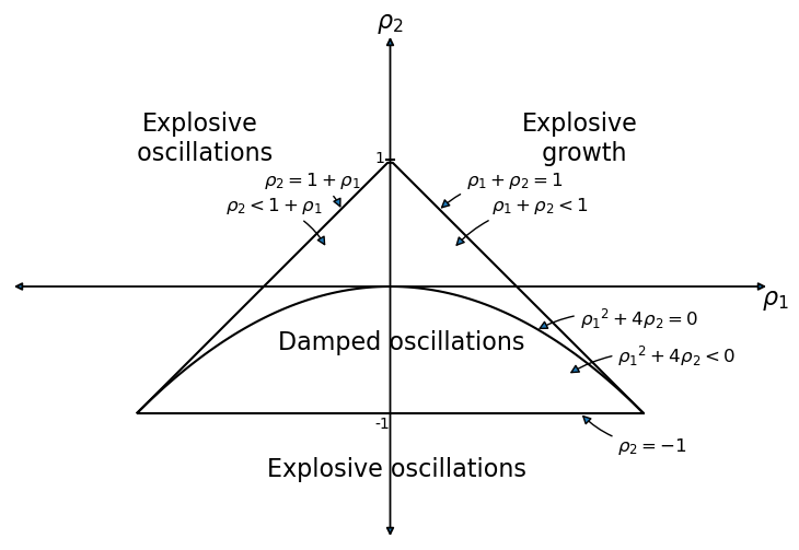
The graph portrays regions in which the \((\lambda_1, \lambda_2)\) root pairs implied by the \((\rho_1 = (\alpha+\beta), \rho_2 = - \beta)\) difference equation parameter pairs in the Samuelson model are such that:
\((\lambda_1, \lambda_2)\) are complex with modulus less than \(1\) - in this case, the \(\{Y_t\}\) sequence displays damped oscillations.
\((\lambda_1, \lambda_2)\) are both real, but one is strictly greater than \(1\) - this leads to explosive growth.
\((\lambda_1, \lambda_2)\) are both real, but one is strictly less than \(-1\) - this leads to explosive oscillations.
\((\lambda_1, \lambda_2)\) are both real and both are less than \(1\) in absolute value - in this case, there is smooth convergence to the steady state without damped cycles.
Later we’ll present the graph with a red mark showing the particular point implied by the setting of \((\alpha,\beta)\).
37.3.1. Function to describe implications of characteristic polynomial#
def categorize_solution(ρ1, ρ2):
    """
    This function takes values of ρ1 and ρ2 and uses them
    to classify the type of solution.
    """
    discriminant = ρ1**2 + 4 * ρ2
    if ρ2 > 1 + ρ1 or ρ2 < -1:
        return "Explosive oscillations"
    elif ρ1 + ρ2 > 1:
        return "Explosive growth"
    elif discriminant < 0:
        return "Damped oscillations"
    else:
        return "Steady state convergence"

def analyze_roots(α, β, verbose=True):
    """
    Unified function to calculate roots and analyze their properties.
    """
    ρ1 = α + β
    ρ2 = -β

    # Compute characteristic polynomial roots
    roots = np.roots([1, -ρ1, -ρ2])

    # Classify solution type
    solution_type = categorize_solution(ρ1, ρ2)

    # Determine root properties
    is_complex = all(isinstance(root, complex) for root in roots)
    is_stable = all(abs(root) < 1 for root in roots)

    if verbose:
        print(f"ρ1 = {ρ1:.2f}, ρ2 = {ρ2:.2f}")
        print(f"Roots: {[f'{root:.2f}' for root in roots]}")
        print(f"Root type: {'Complex' if is_complex else 'Real'}")
        print(f"Stability: {'Stable' if is_stable else 'Unstable'}")
        print(f"Solution type: {solution_type}")

    return {
        'roots': roots,
        'rho1': ρ1,
        'rho2': ρ2,
        'is_complex': is_complex,
        'is_stable': is_stable,
        'solution_type': solution_type
    }
We also write a unified simulation function that can handle both non-stochastic and stochastic versions of the model.
It allows for government spending paths of a few simple forms which
we specify via a dictionary g_params
def simulate_samuelson(
    y_0, y_1, α, β, γ=10, n=100, σ=0, g_params=None, seed=0
):
    """
    Unified simulation function for Samuelson model.

    Parameters:
    g_params: dict with keys 'g', 'g_t', 'duration' for government spending
    seed: random seed for reproducible results
    """
    analysis = analyze_roots(α, β, verbose=False)
    ρ1, ρ2 = analysis['rho1'], analysis['rho2']

    # Initialize time series
    y_t = [y_0, y_1]

    # Generate shocks if stochastic
    if σ > 0:
        np.random.seed(seed)
        ϵ = np.random.normal(0, 1, n)

    # Simulate forward
    for t in range(2, n):

        # Determine government spending
        g = 0
        if g_params:
            g_val, g_t_val = g_params.get('g', 0), g_params.get('g_t', 0)
            duration = g_params.get('duration', None)
            if duration == 'permanent' and t >= g_t_val:
                g = g_val
            elif duration == 'one-off' and t == g_t_val:
                g = g_val
            elif duration is None:
                g = g_val

        # Calculate next value
        y_next = ρ1 * y_t[t-1] + ρ2 * y_t[t-2] + γ + g
        if σ > 0:
            y_next += σ * ϵ[t]

        y_t.append(y_next)

    return y_t, analysis
We will use this function to run simulations of the model.
But before doing that, let’s test the analysis function
analysis = analyze_roots(α=1.3, β=0.4)
ρ1 = 1.70, ρ2 = -0.40
Roots: ['1.42', '0.28']
Root type: Real
Stability: Unstable
Solution type: Explosive growth
37.3.2. Function for plotting paths#
A useful function for our work below is
def plot_y(function=None):
    """Function plots path of Y_t"""

    plt.subplots(figsize=(10, 6))
    plt.plot(function)
    plt.xlabel("$t$")
    plt.ylabel("$Y_t$")
    plt.show()
37.3.3. Manual or “by hand” root calculations#
The following function calculates roots of the characteristic polynomial using high school algebra.
(We’ll calculate the roots in other ways later using analyze_roots.)
The function also plots a \(Y_t\) starting from initial conditions that we set
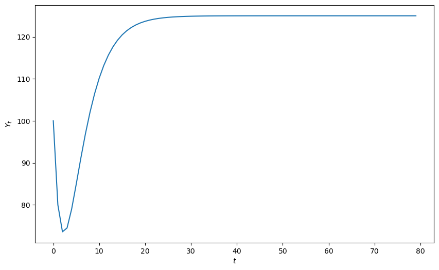
def y_nonstochastic(y_0=100, y_1=80, α=0.92, β=0.5, γ=10, n=80):
"""
This function calculates the roots of the characteristic polynomial
by hand and returns a path of y_t starting from initial conditions
"""
roots = []
ρ1 = α + β
ρ2 = -β
print(f"ρ_1 is {ρ1:.2f}")
print(f"ρ_2 is {ρ2:.2f}")
discriminant = ρ1**2 + 4 * ρ2
if discriminant == 0:
roots.append(-ρ1 / 2)
print("Single real root: ")
print("".join(f"{r:.2f}" for r in roots))
elif discriminant > 0:
roots.append((-ρ1 + sqrt(discriminant).real) / 2)
roots.append((-ρ1 - sqrt(discriminant).real) / 2)
print("Two real roots: ")
print(" ".join(f"{r:.2f}" for r in roots))
else:
roots.append((-ρ1 + sqrt(discriminant)) / 2)
roots.append((-ρ1 - sqrt(discriminant)) / 2)
print("Two complex roots: ")
print(" ".join(f"{r.real:.2f}{r.imag:+.2f}j" for r in roots))
if all(abs(root) < 1 for root in roots):
print("Absolute values of roots are less than one")
else:
print("Absolute values of roots are not less than one")
def transition(x, t):
return ρ1 * x[t - 1] + ρ2 * x[t - 2] + γ
y_t = [y_0, y_1]
for t in range(2, n):
y_t.append(transition(y_t, t))
return y_t
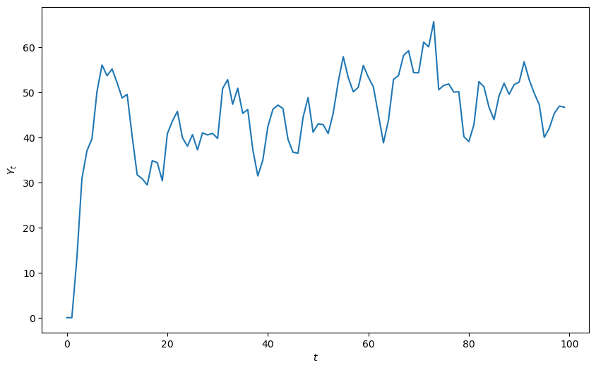
plot_y(y_nonstochastic())
ρ_1 is 1.42
ρ_2 is -0.50
Two real roots:
-0.65 -0.77
Absolute values of roots are less than one
37.3.4. Reverse-engineering parameters to generate damped cycles#
The next cell writes code that takes as inputs the modulus \(r\) and phase \(\phi\) of a conjugate pair of complex numbers in polar form
The code assumes that these two complex numbers are the roots of the characteristic polynomial
It then reverse-engineers \((\alpha,\beta)\) and \((\rho_1, \rho_2)\), pairs that would generate those roots
def f(r, ϕ):
    """
    Takes modulus r and angle ϕ of complex number r exp(j ϕ)
    and creates ρ1 and ρ2 of characteristic polynomial for which
    r exp(j ϕ) and r exp(- j ϕ) are complex roots.

    Returns the multiplier coefficient $\alpha$
    and the accelerator coefficient $\beta$
    that verifies those roots.
    """
    # Create complex conjugate pair from polar coordinates
    g1 = cmath.rect(r, ϕ)
    g2 = cmath.rect(r, -ϕ)

    # Calculate corresponding ρ1, ρ2 parameters
    ρ1 = g1 + g2
    ρ2 = -g1 * g2

    # Derive α and β coefficients from ρ parameters
    β = -ρ2
    α = ρ1 - β
    return ρ1, ρ2, α, β
Now let’s use the function in an example.
Here are the example parameters
r = 0.95

# Cycle period in time units
period = 10
ϕ = 2 * math.pi / period

# Apply the reverse-engineering function
ρ1, ρ2, α, β = f(r, ϕ)

print(f"α, β = {α:.2f}, {β:.2f}")
print(f"ρ1, ρ2 = {ρ1:.2f}, {ρ2:.2f}")
α, β = 0.63+0.00j, 0.90-0.00j
ρ1, ρ2 = 1.54+0.00j, -0.90+0.00j
The real parts of the roots are
print(f"ρ1 = {ρ1.real:.2f}, ρ2 = {ρ2.real:.2f}")
ρ1 = 1.54, ρ2 = -0.90
37.3.5. Root finding using numpy#
Here we’ll use numpy to compute the roots of the characteristic polynomial
r1, r2 = np.roots([1, -ρ1, -ρ2])

p1 = cmath.polar(r1)
p2 = cmath.polar(r2)

print(f"r, ϕ = {r:.2f}, {ϕ:.2f}")
print(f"p1, p2 = ({p1[0]:.2f}, {p1[1]:.2f}), ({p2[0]:.2f}, {p2[1]:.2f})")

print(f"α, β = {α:.2f}, {β:.2f}")
print(f"ρ1, ρ2 = {ρ1:.2f}, {ρ2:.2f}")
r, ϕ = 0.95, 0.63
p1, p2 = (0.95, 0.63), (0.95, -0.63)
α, β = 0.63+0.00j, 0.90-0.00j
ρ1, ρ2 = 1.54+0.00j, -0.90+0.00j
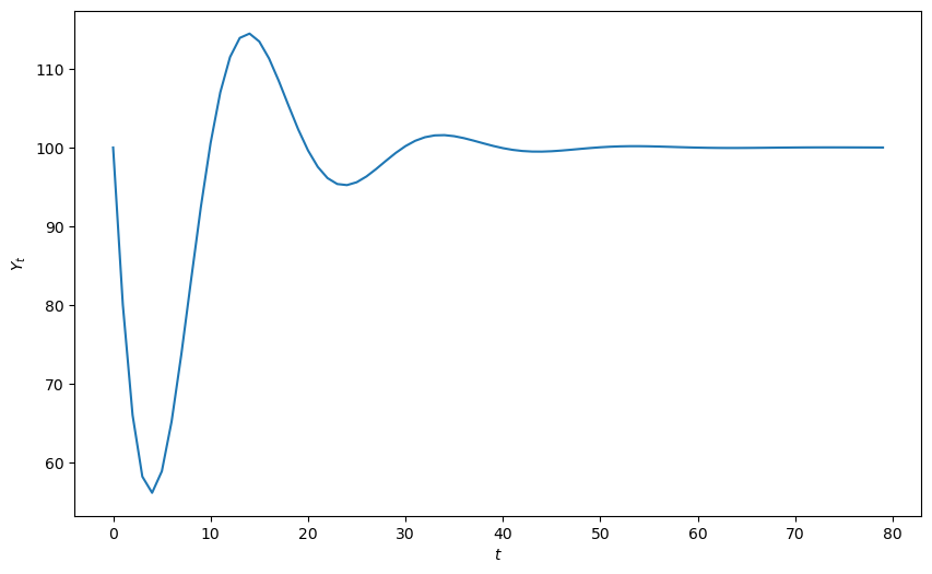
def y_nonstochastic(y_0=100, y_1=80, α=0.9, β=0.8, γ=10, n=80):
    """
    This function enlists numpy to calculate the roots of the characteristic
    polynomial.
    """

    y_series, analysis = simulate_samuelson(y_0, y_1, α, β, γ, n, 0, None, 42)

    print(f"Solution type: {analysis['solution_type']}")
    print(f"Roots are {analysis['roots']}")
    print(f"Root type: {'Complex' if analysis['is_complex'] else 'Real'}")
    print(f"Stability: {'Stable' if analysis['is_stable'] else 'Unstable'}")

    return y_series


plot_y(y_nonstochastic())
Solution type: Damped oscillations
Roots are [0.85+0.27838822j 0.85-0.27838822j]
Root type: Complex
Stability: Stable
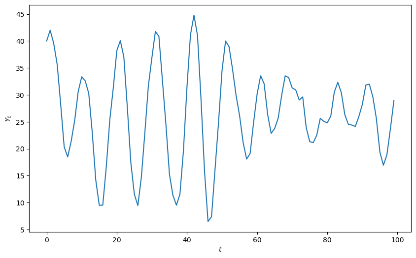
37.3.6. Reverse-engineered complex roots: Example#
The next cell studies the implications of reverse-engineered complex roots.
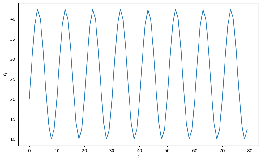
We’ll generate an undamped cycle of period 10
r = 1  # Generates undamped, nonexplosive cycles

period = 10  # Length of cycle in units of time
ϕ = 2 * math.pi / period

# Apply the reverse-engineering function f
ρ1, ρ2, α, β = f(r, ϕ)

# Extract real parts for numerical computation
α = α.real
β = β.real

print(f"α, β = {α:.2f}, {β:.2f}")

ytemp = y_nonstochastic(α=α, β=β, y_0=20, y_1=30)
plot_y(ytemp)
α, β = 0.62, 1.00
Solution type: Damped oscillations
Roots are [0.80901699+0.58778525j 0.80901699-0.58778525j]
Root type: Complex
Stability: Unstable
37.3.7. Digression: Using Sympy to find roots#
We can also use sympy to compute analytic formulas for the roots
init_printing()

r1 = Symbol("ρ_1")
r2 = Symbol("ρ_2")
z = Symbol("z")

sympy.solve(z**2 - r1 * z - r2, z)

α = Symbol("α")
β = Symbol("β")
r1 = α + β
r2 = -β

sympy.solve(z**2 - r1 * z - r2, z)

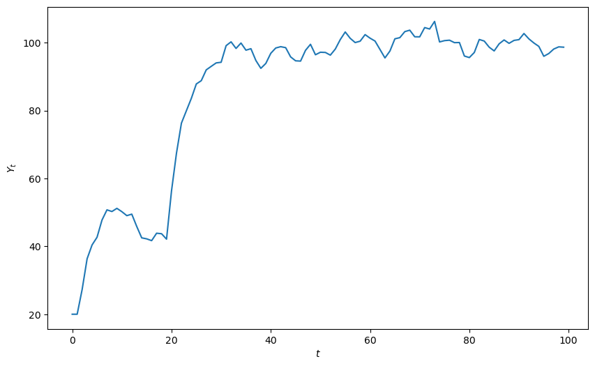
37.4. Stochastic shocks#
Now we’ll construct some code to simulate the stochastic version of the model that emerges when we add a random shock process to aggregate demand
def y_stochastic(y_0=0, y_1=0, α=0.8, β=0.2, γ=10, n=100, σ=5):
    """
    This function takes parameters of a stochastic version of
    the model, analyzes the roots of the characteristic
    polynomial and generates a simulation.
    """

    y_series, analysis = simulate_samuelson(y_0, y_1, α, β, γ, n, σ, None, 42)

    print(f"Solution type: {analysis['solution_type']}")
    print(f"Roots are {[f'{root:.2f}' for root in analysis['roots']]}")
    print(f"Root type: {'Complex' if analysis['is_complex'] else 'Real'}")
    print(f"Stability: {'Stable' if analysis['is_stable'] else 'Unstable'}")

    return y_series


plot_y(y_stochastic())
Solution type: Steady state convergence
Roots are ['0.72', '0.28']
Root type: Real
Stability: Stable
Let’s do a simulation in which there are shocks and the characteristic polynomial has complex roots
r = 0.97

period = 10  # Length of cycle in units of time
ϕ = 2 * math.pi / period

# Apply the reverse-engineering function f
ρ1, ρ2, α, β = f(r, ϕ)

# Extract real parts for numerical computation
α = α.real
β = β.real

print(f"α, β = {α:.2f}, {β:.2f}")
plot_y(y_stochastic(y_0=40, y_1=42, α=α, β=β, σ=2, n=100))
α, β = 0.63, 0.94
Solution type: Damped oscillations
Roots are ['0.78+0.57j', '0.78-0.57j']
Root type: Complex
Stability: Stable
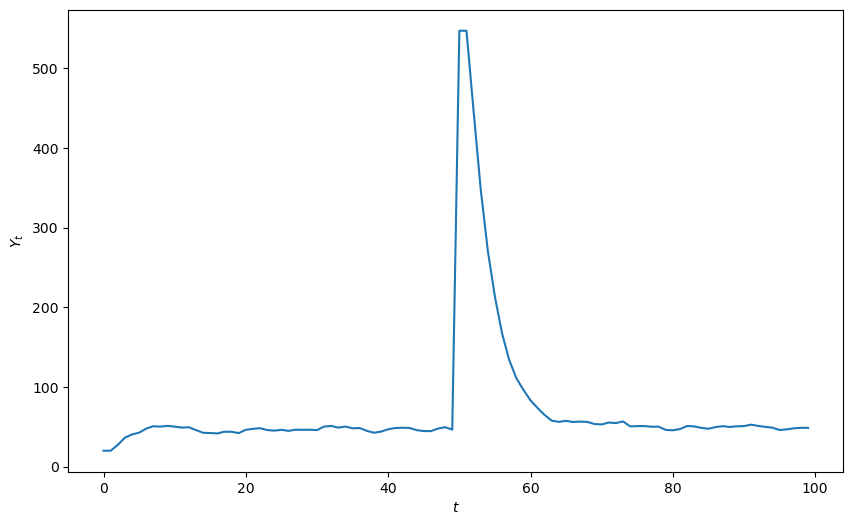
37.5. Government spending#
This function computes a response to either a permanent or one-off increase in government expenditures
def y_stochastic_g(
    y_0=20, y_1=20, α=0.8, β=0.2, γ=10,
    n=100, σ=2, g=0, g_t=0, duration="permanent"
):
    """
    This program computes a response to a permanent increase
    in government expenditures that occurs at time 20
    """

    g_params = (
        {'g': g, 'g_t': g_t, 'duration': duration} if g != 0 else None
    )
    y_series, analysis = simulate_samuelson(
        y_0, y_1, α, β, γ, n, σ, g_params, 42
    )

    print(f"Solution type: {analysis['solution_type']}")
    print(f"Roots: {analysis['roots']}")
    print(f"Root type: {'Complex' if analysis['is_complex'] else 'Real'}")
    print(f"Stability: {'Stable' if analysis['is_stable'] else 'Unstable'}")

    return y_series
A permanent government spending shock can be simulated as follows
plot_y(y_stochastic_g(g=10, g_t=20, duration="permanent"))
Solution type: Steady state convergence
Roots: [0.7236068 0.2763932]
Root type: Real
Stability: Stable
We can also see the response to a one time jump in government expenditures
plot_y(y_stochastic_g(g=500, g_t=50, duration="one-off"))
Solution type: Steady state convergence
Roots: [0.7236068 0.2763932]
Root type: Real
Stability: Stable
37.6. Wrapping everything into a class#
Up to now, we have written functions to do the work.
Now we’ll roll up our sleeves and write a Python class called Samuelson
for the Samuelson model
class Samuelson:
    """
    This class represents the Samuelson model, otherwise known as the
    multiplier-accelerator model.
    The model combines the Keynesian multiplier
    with the accelerator theory of investment.

    The path of output is governed by a linear
    second-order difference equation

    .. math::

        Y_t = \alpha (1 + \beta) Y_{t-1} - \alpha \beta Y_{t-2}

    Parameters
    ----------
    y_0 : scalar
        Initial condition for Y_0
    y_1 : scalar
        Initial condition for Y_1
    α : scalar
        Marginal propensity to consume
    β : scalar
        Accelerator coefficient
    n : int
        Number of iterations
    σ : scalar
        Volatility parameter. It must be greater than or equal to 0. Set
        equal to 0 for a non-stochastic model.
    g : scalar
        Government spending shock
    g_t : int
        Time at which government spending shock occurs. Must be specified
        when duration != None.
    duration : {None, 'permanent', 'one-off'}
        Specifies type of government spending shock. If none, government
        spending equal to g for all t.

    """

    def __init__(
        self, y_0=100, y_1=50,
        α=1.3, β=0.2, γ=10, n=100, σ=0, g=0, g_t=0, duration=None
    ):

        self.y_0, self.y_1, self.α, self.β = y_0, y_1, α, β
        self.n, self.g, self.g_t, self.duration = n, g, g_t, duration
        self.γ, self.σ = γ, σ

        # Use unified analysis function
        self.analysis = analyze_roots(α, β, verbose=False)
        self.ρ1, self.ρ2 = self.analysis['rho1'], self.analysis['rho2']
        self.roots = self.analysis['roots']

    def root_type(self):
        return "Complex conjugate" if self.analysis['is_complex'] else "Real"

    def root_less_than_one(self):
        return self.analysis['is_stable']

    def solution_type(self):
        return self.analysis['solution_type']

    def generate_series(self, seed=0):
        g_params = (
            {'g': self.g, 'g_t': self.g_t, 'duration': self.duration}
            if self.g != 0 else None
        )
        y_series, _ = simulate_samuelson(
            self.y_0, self.y_1, self.α, self.β, self.γ,
            self.n, self.σ, g_params, seed
        )
        return y_series

    def summary(self):
        print("Summary\n" + "-" * 50)
        print(f"Root type: {self.root_type()}")
        print(f"Solution type: {self.solution_type()}")
        print(f"Roots: {str(self.roots)}")

        if self.root_less_than_one() == True:
            print("Absolute value of roots is less than one")
        else:
            print("Absolute value of roots is not less than one")

        if self.σ > 0:
            print("Stochastic series with σ = " + str(self.σ))
        else:
            print("Non-stochastic series")

        if self.g != 0:
            print("Government spending equal to " + str(self.g))

        if self.duration != None:
            print(
                self.duration.capitalize()
                + " government spending shock at t = "
                + str(self.g_t)
            )

    def plot(self, seed=0):
        fig, ax = plt.subplots(figsize=(10, 6))
        ax.plot(self.generate_series(seed))
        ax.set(xlabel="iteration", xlim=(0, self.n))
        ax.set_ylabel("$Y_t$", rotation=0)

        # Display model parameters on the plot
        paramstr = (
            f"$α={self.α:.2f}$ \n $β={self.β:.2f}$ \n "
            f"$\\gamma={self.γ:.2f}$ \n $\\sigma={self.σ:.2f}$ \n "
            f"$\\rho_1={self.ρ1:.2f}$ \n $\\rho_2={self.ρ2:.2f}$"
        )
        props = dict(fc="white", pad=10, alpha=0.5)
        ax.text(
            0.87,
            0.05,
            paramstr,
            transform=ax.transAxes,
            fontsize=12,
            bbox=props,
            va="bottom",
        )

        return fig

    def param_plot(self):


        fig = param_plot()
        ax = fig.gca()

        # Display eigenvalues in the legend
        for i, root in enumerate(self.roots):
            if isinstance(root, complex):

                # Handle sign formatting for complex number display
                operator = ["+", ""]
                root_real = self.roots[i].real
                root_imag = self.roots[i].imag
                label = (
                    rf"$\lambda_{i+1} = {root_real:.2f}"
                    rf"{operator[i]} {root_imag:.2f}i$"
                )
            else:
                label = rf"$\lambda_{i+1} = {self.roots[i].real:.2f}$"

            # Add invisible point for legend entry
            ax.scatter(
                0, 0, s=0, label=label
            )

        # Mark current parameter values on the stability diagram
        ax.scatter(
            self.ρ1,
            self.ρ2,
            s=100,
            c="red",
            marker="+",
            label=r"$(\rho_1, \rho_2)$",
            zorder=5,
        )

        plt.legend(fontsize=12, loc=3)

        return fig
37.6.1. Illustration of Samuelson class#
Now we’ll put our Samuelson class to work on an example
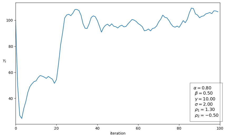
sam = Samuelson(α=0.8, β=0.5, σ=2, g=10, g_t=20, duration="permanent")
sam.summary()
Summary
--------------------------------------------------
Root type: Complex conjugate
Solution type: Damped oscillations
Roots: [0.65+0.27838822j 0.65-0.27838822j]
Absolute value of roots is less than one
Stochastic series with σ = 2
Government spending equal to 10
Permanent government spending shock at t = 20
sam.plot()
plt.show()
37.6.2. Using the graph#
We’ll use our graph to show where the roots lie and how their location is consistent with the behavior of the path just graphed.
The red \(+\) sign shows the location of the roots
sam.param_plot()
plt.show()
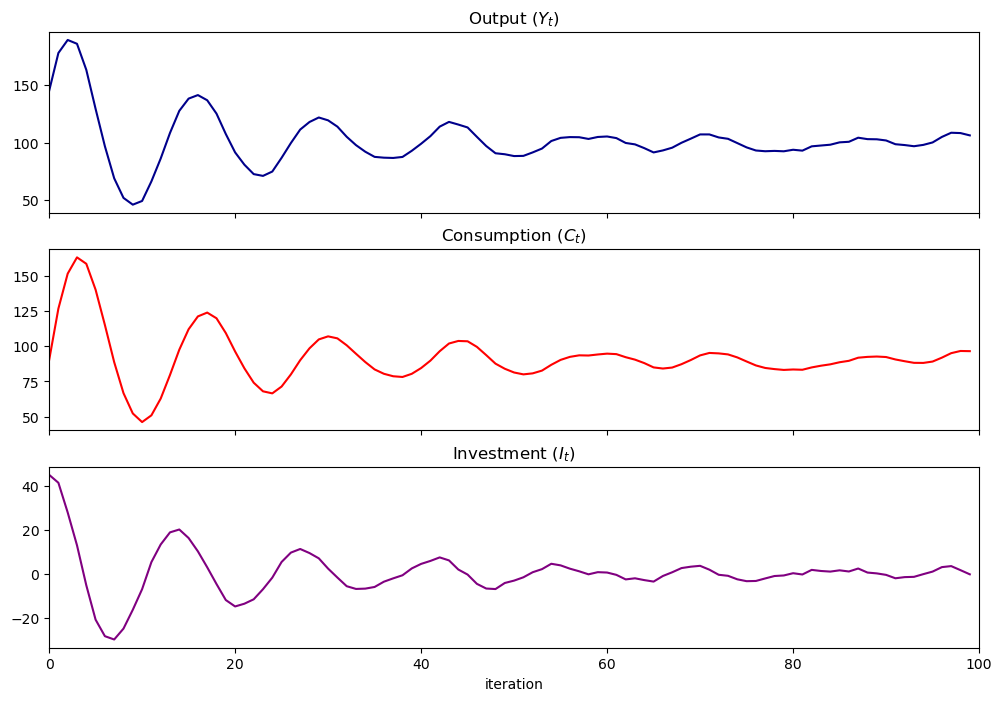
37.7. Using the LinearStateSpace class#
It turns out that we can use the QuantEcon.py LinearStateSpace class to do much of the work that we have done from scratch above.
Here is how we map the Samuelson model into an instance of a
LinearStateSpace class
α = 0.8
β = 0.9
ρ1 = α + β
ρ2 = -β
γ = 10
σ = 1
g = 10
n = 100

A = [[1, 0, 0], [γ + g, ρ1, ρ2], [0, 1, 0]]

G = [
    [γ + g, ρ1, ρ2],  # Y_{t+1}
    [γ, α, 0],        # C_{t+1}
    [0, β, -β],       # I_{t+1}
]

μ_0 = [1, 100, 50]
C = np.zeros((3, 1))
C[1] = σ  # Shock variance

sam_t = LinearStateSpace(A, C, G, mu_0=μ_0)

x, y = sam_t.simulate(ts_length=n)

fig, axes = plt.subplots(3, 1, sharex=True, figsize=(12, 8))
titles = ["Output ($Y_t$)", "Consumption ($C_t$)", "Investment ($I_t$)"]
colors = ["darkblue", "red", "purple"]
for ax, series, title, color in zip(axes, y, titles, colors):
    ax.plot(series, color=color)
    ax.set(title=title, xlim=(0, n))

axes[-1].set_xlabel("iteration")

plt.show()
37.7.1. Other methods in the LinearStateSpace class#
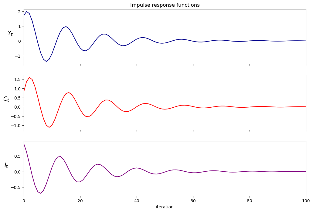
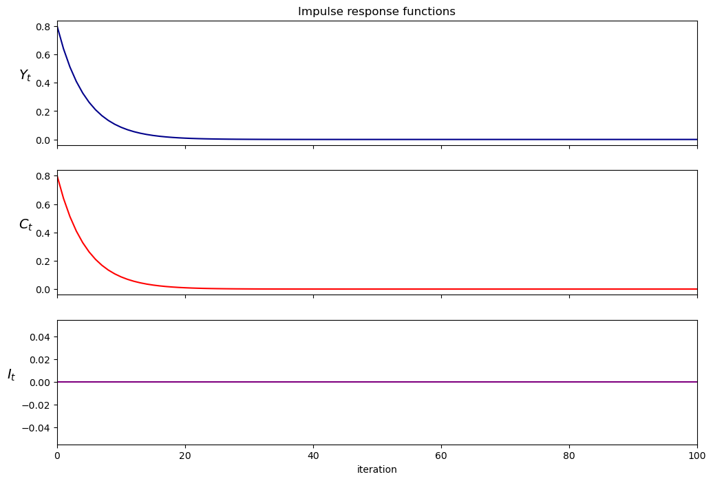
Let’s plot impulse response functions for the instance of the
Samuelson model using a method in the LinearStateSpace class
imres = sam_t.impulse_response()
imres = np.asarray(imres)
y1 = imres[:, :, 0]
y2 = imres[:, :, 1]
y1.shape

Now let’s compute the zeros of the characteristic polynomial by simply calculating the eigenvalues of \(A\)
A = np.asarray(A)
w, v = np.linalg.eig(A)
print(np.round(w, 2))
[0.85+0.42j 0.85-0.42j 1. +0.j ]
37.7.2. Inheriting methods from LinearStateSpace#
We could also create a subclass of LinearStateSpace (inheriting all its
methods and attributes) to add more functions to use
class SamuelsonLSS(LinearStateSpace):
    """
    This subclass creates a Samuelson multiplier-accelerator model
    as a linear state space system.
    """

    def __init__(self, y_0=100, y_1=50, α=0.8, β=0.9, γ=10, σ=1, g=10):

        self.α, self.β = α, β
        self.y_0, self.y_1, self.g = y_0, y_1, g
        self.γ, self.σ = γ, σ

        # Set initial state vector
        self.initial_μ = [1, y_0, y_1]

        self.ρ1 = α + β
        self.ρ2 = -β

        # Construct state transition matrix
        self.A = [[1, 0, 0], [γ + g, self.ρ1, self.ρ2], [0, 1, 0]]

        # Construct observation matrix
        self.G = [
            [γ + g, self.ρ1, self.ρ2],  # Y_{t+1}
            [γ, α, 0],                  # C_{t+1}
            [0, β, -β],                 # I_{t+1}
        ]

        self.C = np.zeros((3, 1))
        self.C[1] = σ  # Shock variance

        # Initialize the LinearStateSpace instance
        LinearStateSpace.__init__(
            self, self.A, self.C, self.G, mu_0=self.initial_μ
        )

    # Create unicode aliases for mu_0 and Sigma_0 in the parent class
    @property
    def μ_0(self):
        return self.mu_0

    @μ_0.setter
    def μ_0(self, value):
        self.mu_0 = value

    @property
    def Σ_0(self):
        return self.Sigma_0

    @Σ_0.setter
    def Σ_0(self, value):
        self.Sigma_0 = value

    def plot_simulation(self, ts_length=100, stationary=True, seed=0):

        # Store original distribution parameters
        temp_μ = self.μ_0
        temp_Σ = self.Σ_0

        # Use stationary distribution for simulation
        if stationary == True:
            try:
                (self.μ_x, self.μ_y, self.Σ_x, self.Σ_y, self.Σ_yx
                ) = self.stationary_distributions()
                self.μ_0 = self.μ_x
                self.Σ_0 = self.Σ_x

            # Handle case where stationary distribution doesn't exist
            except ValueError:
                print("Stationary distribution does not exist")

        np.random.seed(seed)
        x, y = self.simulate(ts_length)

        fig, axes = plt.subplots(3, 1, sharex=True, figsize=(12, 8))
        titles = ["Output ($Y_t$)",
                  "Consumption ($C_t$)",
                  "Investment ($I_t$)"]
        colors = ["darkblue", "red", "purple"]
        for ax, series, title, color in zip(axes, y, titles, colors):
            ax.plot(series, color=color)
            ax.set(title=title, xlim=(0, n))

        axes[-1].set_xlabel("iteration")
        plt.show()

        # Restore original distribution parameters
        self.μ_0 = temp_μ
        self.Σ_0 = temp_Σ

    def plot_irf(self, j=5):

        x, y = self.impulse_response(j)

        # Reshape impulse responses for plotting
        yimf = np.array(y).flatten().reshape(j + 1, 3).T

        fig, axes = plt.subplots(3, 1, sharex=True, figsize=(12, 8))
        labels = ["$Y_t$", "$C_t$", "$I_t$"]
        colors = ["darkblue", "red", "purple"]
        for ax, series, label, color in zip(axes, yimf, labels, colors):
            ax.plot(series, color=color)
            ax.set(xlim=(0, j))
            ax.set_ylabel(label, rotation=0, fontsize=14, labelpad=10)

        axes[0].set_title("Impulse response functions")
        axes[-1].set_xlabel("iteration")
        plt.show()

    def multipliers(self, j=5):
        x, y = self.impulse_response(j)
        return np.sum(np.array(y).flatten().reshape(j + 1, 3), axis=0)
37.7.3. Illustrations#
Let’s show how we can use the SamuelsonLSS
samlss = SamuelsonLSS()
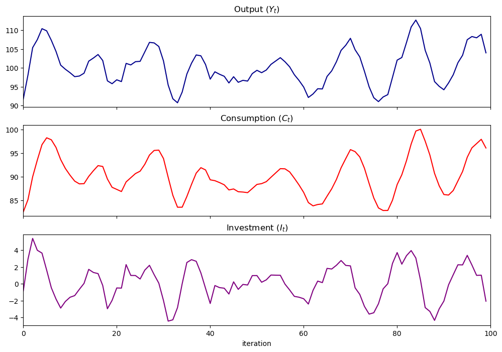
samlss.plot_simulation(100, stationary=False)
plt.show()
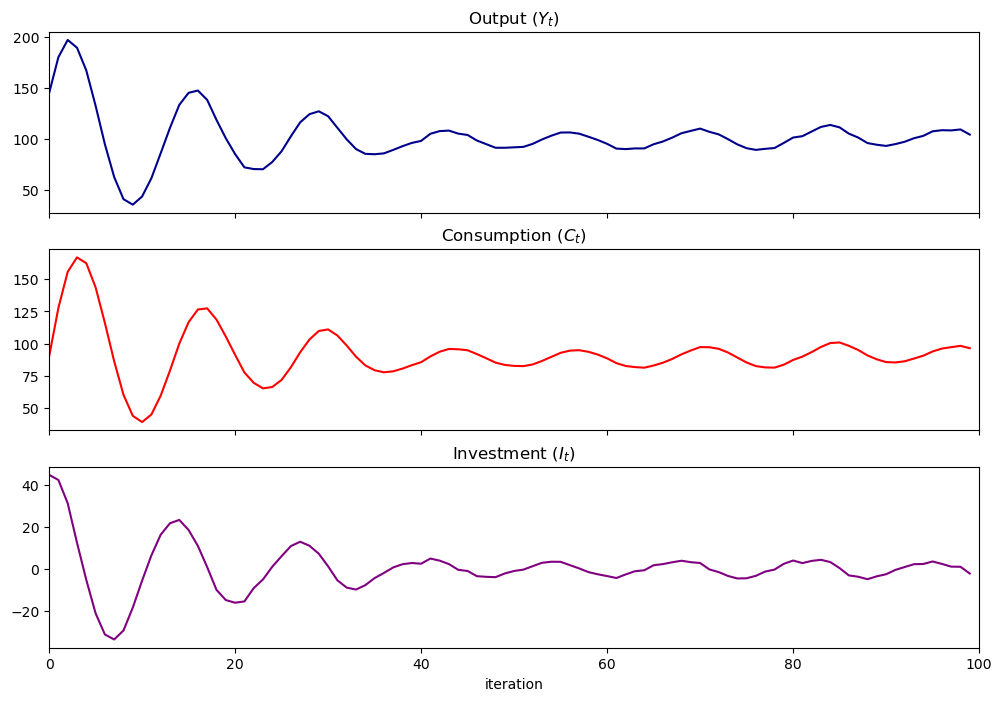
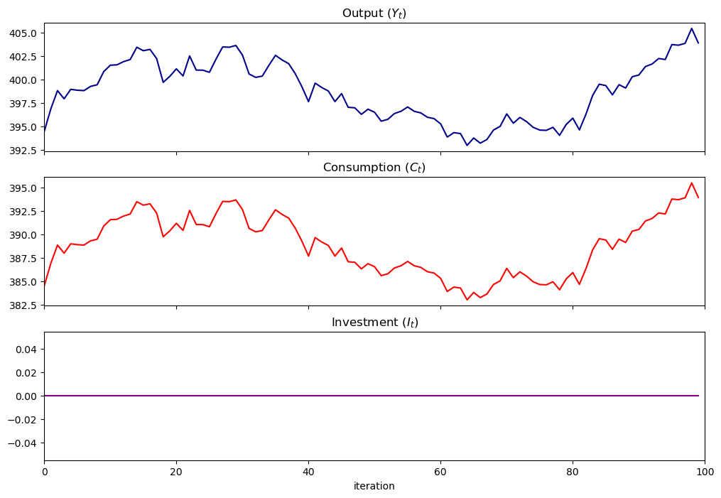
samlss.plot_simulation(100, stationary=True)
plt.show()
samlss.plot_irf(100)
plt.show()
samlss.multipliers()
array([7.414389, 6.835896, 0.578493])
37.8. Pure multiplier model#
Let’s shut down the accelerator by setting \(b=0\) to get a pure multiplier model
the absence of cycles gives an idea about why Samuelson included the accelerator
pure_multiplier = SamuelsonLSS(α=0.95, β=0)
pure_multiplier.plot_simulation()
pure_multiplier = SamuelsonLSS(α=0.8, β=0)
pure_multiplier.plot_simulation()
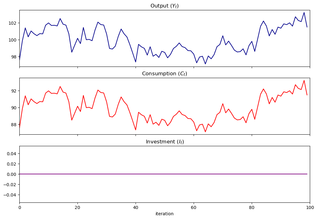
pure_multiplier.plot_irf(100)
37.9. Summary#
In this lecture, we wrote functions and classes to represent non-stochastic and stochastic versions of the Samuelson (1939) multiplier-accelerator model, described in [Samuelson, 1939].
We saw that different parameter values led to different output paths, which could either be stationary, explosive, or oscillating.
We also were able to represent the model using the QuantEcon.py LinearStateSpace class.